


-
作为典型的单中子晕核, 11Be在原子及核物理研究中具有独特的意义. 本文针对类氦11Be2+离子, 采用相对论组态相互作用方法, 高精度计算了主量子数最高达$n = 8$的$n^{3}{\mathrm{S}}_1$和$n^{3}{\mathrm{P}}_{0,1,2}$态的能量与波函数. 通过将有限核质量修正算符直接引入Dirac-Coulomb-Breit哈密顿量, 使计算能够同时考虑相对论效应和质量相关修正. 基于计算的高精度能量与波函数, 本文进一步确定了$k^3{\mathrm{S}}_1 \rightarrow m^3{\mathrm{P}}_{0,1,2}$ ($k \leqslant 5$, $m \leqslant 8$)电偶极跃迁的振子强度, 精度达3—6位有效数字. 此外, 利用态求和法计算了$n'^3{\mathrm{S}}_1$ ($n' \leqslant 5$)态在宽光子频率范围内的动力学电偶极极化率, 在远离共振位置处结果最高可达10–6精度水平. 上述高精度计算结果为11Be2+离子在高精度测量中涉及的斯塔克频移评估以及光与物质相互作用的模拟等方面提供了重要的理论依据和关键输入参数.
11Be, as a typical one-neutron halo nucleus, is of unique significance in studying atomic and nuclear physics. The nucleus comprises a tightly bound 10Be core and a loosely bound valence neutron, forming an exotic nuclear configuration that is significantly different from traditional nuclear configuration in both magnetic and charge radii, thereby establishing a unique platform for investigating nuclear-electron interactions. In this study, we focus on the helium-like 11Be2+ ion and systematically calculate the energies and wavefunctions of the $n^{3}S_1$ and $n^{3}{\mathrm{P}}_{0,1,2}$ states up to principal quantum number $n=8$ by employing the relativistic configuration interaction (RCI) method combined with high-order B-spline basis functions. By directly incorporating the nuclear mass shift operator $H_{\mathrm{M}}$ into the Dirac-Coulomb-Breit (DCB) Hamiltonian, we comprehensively investigate the relativistic effects, Breit interactions, and nuclear mass corrections for 11Be2+. The results demonstrate that the energies of states with $n\leqslant 5$ converge to eight significant digits, showing excellent agreement with existing NRQED values, such as $-9.29871191(5)$ a.u. for the $^{3}{\mathrm{S}}_1$ state. The nuclear mass corrections are on the order of 10–4 a.u. and decrease with principal quantum number increasing. By using the high-precision wavefunctions, the electric dipole oscillator strengths for $k^3{\mathrm{S}}_1 \rightarrow m^3{\mathrm{P}}_{0,1,2}$ transitions ($k \leqslant 5$, $m \leqslant 8$) are determined, resulting in low-lying excited states ($m\leqslant4$) accurate to six significant digits, thereby providing reliable data for evaluating transition probabilities and radiative lifetimes. Furthermore, the dynamic electric dipole polarizabilities of the $n'^3{\mathrm{S}}_1$ ($n' \leqslant 5$) states are calculated using the sum-over-states method. The static polarizabilities exhibit a significant increase with principal quantum number increasing. For the $J=1$ state, the difference in polarizability between the magnetic sublevels $M_J=0$ and $M_J=\pm1$ is three times the tensor polarizability. In the calculation of dynamic polarizabilities, the precision reaches 10–6 in non-resonant regions, whereas achieving the same accuracy near resonance requires higher energy precision. These high-precision computational results provide crucial theoretical foundations and key input parameters for evaluating Stark shifts in high-precision measurements, simulating light-matter interactions, and investigating single-neutron halo nuclear structures. 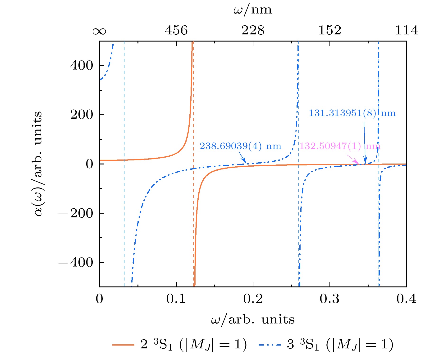
[1] [2] [3] [4] [5] [6] [7] [8] [9] [10] [11] [12] [13] [14] [15] [16] [17] [18] [19] [20] [21] [22] [23] [24] [25] [26] [27] [28] [29] [30] [31] [32] [33] [34] [35] -
(N, $ \ell_m $) $ 2 ^3\mathrm{S}_1 $ $ 3 ^3\mathrm{S}_1 $ $ 4 ^3\mathrm{S}_1 $ $ 5 ^3\mathrm{S}_1 $ $ 6 ^3\mathrm{S}_1 $ $ 7 ^3\mathrm{S}_1 $ $ 8 ^3\mathrm{S}_1 $ (40, 8) –9.2987118781 –8.5483475380 –8.3017888508 –8.1909936393 –8.1318566822 –8.0966153793 –8.0739367761 (40, 9) –9.2987119119 –8.5483475470 –8.3017888543 –8.1909936410 –8.1318566832 –8.0966153799 –8.0739367765 (40, 10) –9.2987118673 –8.5483475442 –8.3017888537 –8.1909936408 –8.1318566831 –8.0966153798 –8.0739367764 (45, 10) –9.298 711 9028 –8.5483475516 –8.3017888542 –8.1909936238 –8.1318565642 –8.0966147583 –8.0739335599 (50, 10) –9.2987118649 –8.5483475498 –8.3017888539 –8.1909936224 –8.1318565546 –8.0966147052 –8.0739332679 Extrap. –9.29871191(5) –8.54834755(2) –8.30178885(1) –8.19099362(3) –8.1318566(1) –8.0966147(4) –8.073933(4) –9.298711181[21] ∞Be2+ –9.29917621(4)[29] –8.54877343(4)[29] –8.30220222(4)[29] –8.19140139(4)[29] –8.1322613(2) –8.0970178(6) –8.074334(5)  下载: 导出CSV
n $ ^3{\mathrm{P}}_0 $(11Be2+) $ ^3{\mathrm{P}}_0 $(∞Be2+) $ ^3{\mathrm{P}}_1 $(11Be2+) $ ^3{\mathrm{P}}_1 $(∞Be2+) $ ^3{\mathrm{P}}_2 $(11Be2+) $ ^3{\mathrm{P}}_2 $(∞Be2+) 2 –9.17627904(4) –9.176 700 64(4)[29] –9.17633162(4) –9.17675322(4)[29] –9.17626402(4) –9.17668561(4)[29] –9.176278322[21] –9.176330730[21] –9.176263355[21] 3 –8.51591623(4) –8.51633141(4)[29] –8.51592914(4) –8.51634433(4)[29] –8.51590908(4) –8.51632431(4)[29] 4 –8.28867151(4) –8.28908063(4)[29] –8.28867658(4) –8.28908570(4)[29] –8.28866814(4) –8.28907727(4)[29] 5 –8.18442245(4) –8.18482810(4)[29] –8.18442495(4) –8.18483061(4)[29] –8.18442064(4) –8.18482630(4)[29] 6 –8.12810385(8) –8.12850744(8) –8.12810527(8) –8.12850886(8) –8.12810278(8) –8.12850637(8) 7 –8.09427236(8) –8.09467469(8) –8.09427324(8) –8.09467556(8) –8.0942717(1) –8.0946740(1) 8 –8.0723741(4) –8.0727757(4) –8.0723745(4) –8.0727762(4) –8.072373(4) –8.0727752(4)
下载: 导出CSV
$ 2 ^3{\mathrm{S}}_1 $ $ 3 ^3{\mathrm{S}}_1 $ $ 4 ^3{\mathrm{S}}_1 $ $ 5 ^3{\mathrm{S}}_1 $ $ 2^3{\mathrm{P}}_0 $ 2.372207(2)[–2] 9.872733(2)[–3] 1.928282(2)[–3] 7.371365(4)[–4] $ 2^3{\mathrm{P}}_1 $ 7.113520(4)[–2] 2.959444(1)[–2] 5.780477(2)[–3] 2.209758(2)[–3] $ 2^3{\mathrm{P}}_2 $ 1.186353(6)[–1] 4.935354(6)[–2] 9.638898(6)[–3] 3.684637(4)[–3] $ 3^3{\mathrm{P}}_0 $ 2.8034387(2)[–2] 3.9595500(4)[–2] 2.1969329(1)[–2] 4.408759(2)[–3] $ 3^3{\mathrm{P}}_1 $ 8.412570(1)[–2] 1.1872683(2)[–1] 6.5866197(8)[–2] 1.3218516(4)[–2] $ 3^3{\mathrm{P}}_2 $ 1.4016114(8)[–1] 1.980174(5)[–1] 1.0983887(8)[–1] 2.204119(1)[–2] $ 4^3{\mathrm{P}}_0 $ 7.9394418(4)[–3] 2.9307965(4)[–2] 5.442867(2)[–2] 3.485147(2)[–2] $ 4^3{\mathrm{P}}_1 $ 2.3822715(1)[–2] 8.794741(2)[–2] 1.6320086(4)[–2] 1.0449598(8)[–1] $ 4^3{\mathrm{P}}_2 $ 3.969574(2)[–2] 1.465153(2)[–1] 2.721986(4)[–1] 1.742527(2)[–1] $ 5^3{\mathrm{P}}_0 $ 3.436979(4)[–3] 8.804208(4)[–3] 3.165094(4)[–2] 6.89132(2)[–2] $ 5^3{\mathrm{P}}_1 $ 1.031254(1)[–2] 2.641763(1)[–2] 9.49775(1)[–2] 2.066303(6)[–1] $ 5^3{\mathrm{P}}_2 $ 1.718454(2)[–2] 4.401593(4)[–2] 1.582203(2)[–1] 3.446360(4)[–1] $ 6^3{\mathrm{P}}_0 $ 1.822257(8)[–3] 3.98831(2)[–3] 9.67922(2)[–3] 3.44362(4)[–2] $ 6^3{\mathrm{P}}_1 $ 5.46755(4)[–3] 1.196685(8)[–2] 2.904307(4)[–2] 1.03336(2)[–1] $ 6^3{\mathrm{P}}_2 $ 9.11117(6)[–3] 1.99396(1)[–2] 4.838841(4)[–2] 1.72139(1)[–1] $ 7^3{\mathrm{P}}_0 $ 1.08963(8)[–3] 2.1925(2)[–3] 4.4708(2)[–3] 1.057500(8)[–2] $ 7^3{\mathrm{P}}_1 $ 3.2693(2)[–3] 6.5784(6)[–3] 1.34147(8)[–2] 3.17309(6)[–2] $ 7^3{\mathrm{P}}_2 $ 5.4481(6)[–3] 1.0961(1)[–2] 2.2351(1)[–2] 5.2866(2)[–2] $ 8^3{\mathrm{P}}_0 $ 7.067(8)[–4] 1.350(1)[–3] 2.503(4)[–3] 4.926(4)[–3] $ 8^3P_1 $ 2.1182(4)[–3] 4.051(4)[–3] 7.510(4)[–3] 1.479(2)[–3] $ 8^3{\mathrm{P}}_2 $ 3.530(2)[–3] 6.750(2)[–3] 1.252(2)[–2] 2.464(2)[–2]
下载: 导出CSV
(N, $ \ell_m $) $ 2\, ^3 {\mathrm{S}}_1(M_{J}=0/\pm 1) $ $ 3\, ^3 {\mathrm{S}}_1(M_{J}=0/\pm 1) $ $ 4\, ^3 {\mathrm{S}}_1(M_{J}=0/\pm 1) $ $ 5\, ^3 {\mathrm{S}}_1(M_{J}=0/\pm 1) $ (40, 8) 14.888529/14.891730 343.889786/343.954302 2868.6928/2869.2072 14424.502/14427.048 (40, 9) 14.888533/14.891735 343.889940/343.954462 2868.6941/2869.2085 14424.508/14427.054 (40, 10) 14.888538/14.891742 343.890034/343.954574 2868.6946/2869.2092 14424.510/14427.058 (45, 10) 14.888561/14.891758 343.890263/343.954742 2868.6970/2869.2111 14424.544/14427.088 (50, 10) 14.888528/14.891735 343.889933/343.954502 2868.6944/2869.2092 14424.531/14427.080 Extrap. 14.88858(6)/14.89177(4) 343.8904(7)/343.9548(5) 2868.697(5)/2869.211(4) 14424.54(4)/14427.08(4)
下载: 导出CSV
ω/a.u. $ 2 ^3\mathrm{S}_1(M_{J}=0/\pm 1) $ $ 3 ^3\mathrm{S}_1(M_{J}=0/\pm 1) $ $ 4 ^3\mathrm{S}_1(M_{J}=0/\pm 1) $ $ 5 ^3\mathrm{S}_1(M_{J}=0/\pm 1) $ 0.02 15.27929(3)/15.28277(2) 551.7125(9)/551.9742(7) –2126.974(5)/–2125.537(4) –1666.090(2)/–1665.446(2) 0.03 15.79888(3)/15.80274(3) 2348.47(3)/2355.50(2) –649.2535(8)/–648.9762(6) –638.422(2)/–638.155(2) 0.04 16.59145(4)/16.59592(3) –645.258(3)/–644.484(2) –317.9701(4)/–317.8436(3) –284.578(3)/–284.410(3) 0.045 17.11436(4)/17.11926(3) –361.0677(9)/–360.7746(7) –238.3984(3)/–238.3025(2) –171.451(4)/–171.301(4) 0.05 17.74088(4)/17.74631(3) –240.8547(5)/–240.6914(4) –183.3957(2)/–183.3195(2) –60.173(6)/–60.025(7) 0.055 18.49116(5)/18.49728(4) –175.3147(3)/–175.2190(3) –143.3993(2)/–143.3365(2) 102.35(2)/102.53(2) 0.06 19.39221(5)/19.39919(4) –134.5050(2)/–134.4378(2) –113.0578(2)/–113.00454(9) 672.43(7)/672.93(7) 0.065 20.48070(6)/20.48879(5) –106.9053(2)/–106.8553(2) –89.1419(1)/–89.09557(8) –1326.21(8)/–1325.85(8) 0.07 21.80763(7)/21.81719(6) –87.1505(2)/–87.11157(9) –69.56520(9)/–69.52388(6) –490.156(5)/–490.103(5) 0.075 23.44577(9)/23.45730(7) –72.41078(9)/–72.37938(7) –52.87530(8)/–52.83766(5) –338.839(2)/–338.785(2) 0.08 25.5025(2)/25.51673(8) –61.05605(8)/–61.03007(6) –37.95614(6)/–37.92106(5) –278.694(3)/–278.627(3) 0.085 28.1427(2)/28.1609(1) –52.08358(7)/–52.06161(5) –23.81351(7)/–23.77994(6) –257.546(6)/–257.452(6) 0.09 31.6335(2)/31.6576(2) –44.84405(6)/–44.82516(4) –9.35342(8)/–9.32025(7) –277.90(2)/–277.68(2) 0.095 36.4367(3)/36.4702(2) –38.89943(5)/–38.88295(4) 6.9806(1)/7.01487(9) –432.7(2)/–431.7(2) 0.10 43.4261(4)/43.4760(3) –33.94404(5)/–33.92949(4) 28.0790(2)/28.1170(2) 441.99(6)/442.72(6) 0.11 74.483(2)/74.6458(9) –26.18144(4)/–26.16973(3) 131.7548(7)/131.8358(8) 32.52(3)/32.53(3) 0.12 361.19(4)/365.51(3) –20.39655(3)/–20.38682(2) –486.980(5)/–486.775(5) –146(1)/–146(1) 0.13 –111.268(4)/–110.830(3) –15.91658(3)/–15.90826(2) –116.4122(2)/–116.4040(2) –8.5(2)/–8.4(2) 0.14 –45.6790(6)/–45.5965(5) –12.32375(2)/–12.31647(2) –68.80539(6)/–68.79816(6) 0.15 –27.7762(3)/–27.7422(2) –9.34226(2)/–9.33576(2) –46.6878(2)/–46.6794(2) 0.16 –19.4618(2)/–19.4433(1) –6.77800(2)/–6.77207(2) –28.4859(4)/–28.4748(4) 0.17 –14.68262(9)/–14.67079(7) –4.48302(2)/–4.47750(2) 27.568(5)/27.602(5) 0.18 –11.59257(6)/–11.58420(5) –2.33146(2)/–2.32622(1) –76.562(2)/–76.550(2) 0.19 –9.43904(5)/–9.43342(4) –0.19850(2)/–0.193392(9) –51.2307(7)/–51.2156(7) 0.20 –7.85783(4)/–7.85328(3) 2.06578(2)/2.070910(9) –47.611(3)/–47.577(3) 0.22 –5.70307(3)/–5.70005(2) 8.05211(2)/8.058053(9) 56.557(6)/56.635(6) 0.24 –4.31412(2)/–4.31196(2) 22.40003(2)/22.41095(2) 2.70(5)/2.70(5) 0.26 –3.35158(2)/–3.349930(9) –1580.80(4)/–1566.25(4) –5.1(6)/–5.0(6) 0.28 –2.64914(1)/–2.647830(7) –26.249939(7)/–26.248577(8) 0.30 –2.115953(8)/–2.114877(6) –12.800496(3)/–12.799903(3) 0.32 –1.698284(7)/–1.697376(5) –7.278323(3)/–7.277525(3) 0.34 –1.362367(6)/–1.361585(4) –2.571976(7)/–2.570642(7) 0.36 –1.085927(5)/–1.085241(4) 22.4313(3)/22.4461(3) 0.38 –0.853663(4)/–0.853051(3) –10.49399(3)/–10.49349(3) 0.40 –0.654682(4)/–0.654128(3) –4.67869(3)/–4.67806(3)
下载: 导出CSV
-
[1] [2] [3] [4] [5] [6] [7] [8] [9] [10] [11] [12] [13] [14] [15] [16] [17] [18] [19] [20] [21] [22] [23] [24] [25] [26] [27] [28] [29] [30] [31] [32] [33] [34] [35]


 下载:
下载:

计量
- 文章访问数: 1538
- PDF下载量: 37
- 被引次数: 0